Deconvolution of PBMC Data
Introduction
This demo shows the Statescope workflow on PBMC bulk data. The process includes:
- Importing libraries and loading a bulk dataset.
- Initializing the Statescope model.
- Running deconvolution, refinement, and state discovery.
- Visualizing the results with:
- A heatmap of cell type fractions,
- A plot of cophenetic coefficients,
- A bar plot of state loadings.
Step 1: Import Libraries
import Statescope.Statescope as scope
import pandas as pd
Step 2: Load the Bulk Dataset
# Read bulk dataset GSE263756
Bulk = pd.read_csv(
    'https://github.com/tgac-vumc/StatescopeData/raw/refs/heads/main/Bulk/PBMC/GSE263756.txt',
    sep='\t',
    index_col='Geneid'
)
Bulk.head(3)
Step 3: Initialize the Statescope Model
Statescope_model = scope.Initialize_Statescope(Bulk, TumorType='PBMC', Ncelltypes=7)
Step 4: Run Deconvolution
Statescope_model.Deconvolution()
Console output shows that deconvolution completed successfully.
Step 5: Run Refinement
Statescope_model.Refinement()
Console output shows that refinement completed successfully.
Step 6: Run StateDiscovery
Statescope_model.StateDiscovery()
Console output shows that state discovery completed successfully.
Step 7: Visualize Results
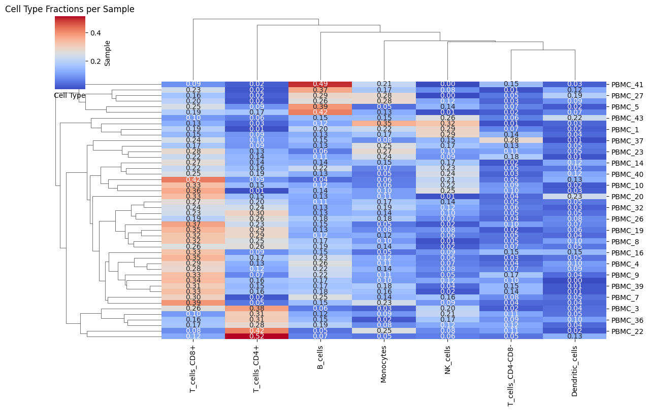
7.1: Heatmap of Cell Type Fractions
from Statescope.Statescope import Heatmap_Fractions
Heatmap_Fractions(Statescope_model)
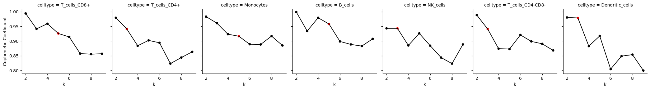
7.2: Cophenetic Coefficients Plot
from Statescope.Statescope import Plot_CopheneticCoefficients
Plot_CopheneticCoefficients(Statescope_model)
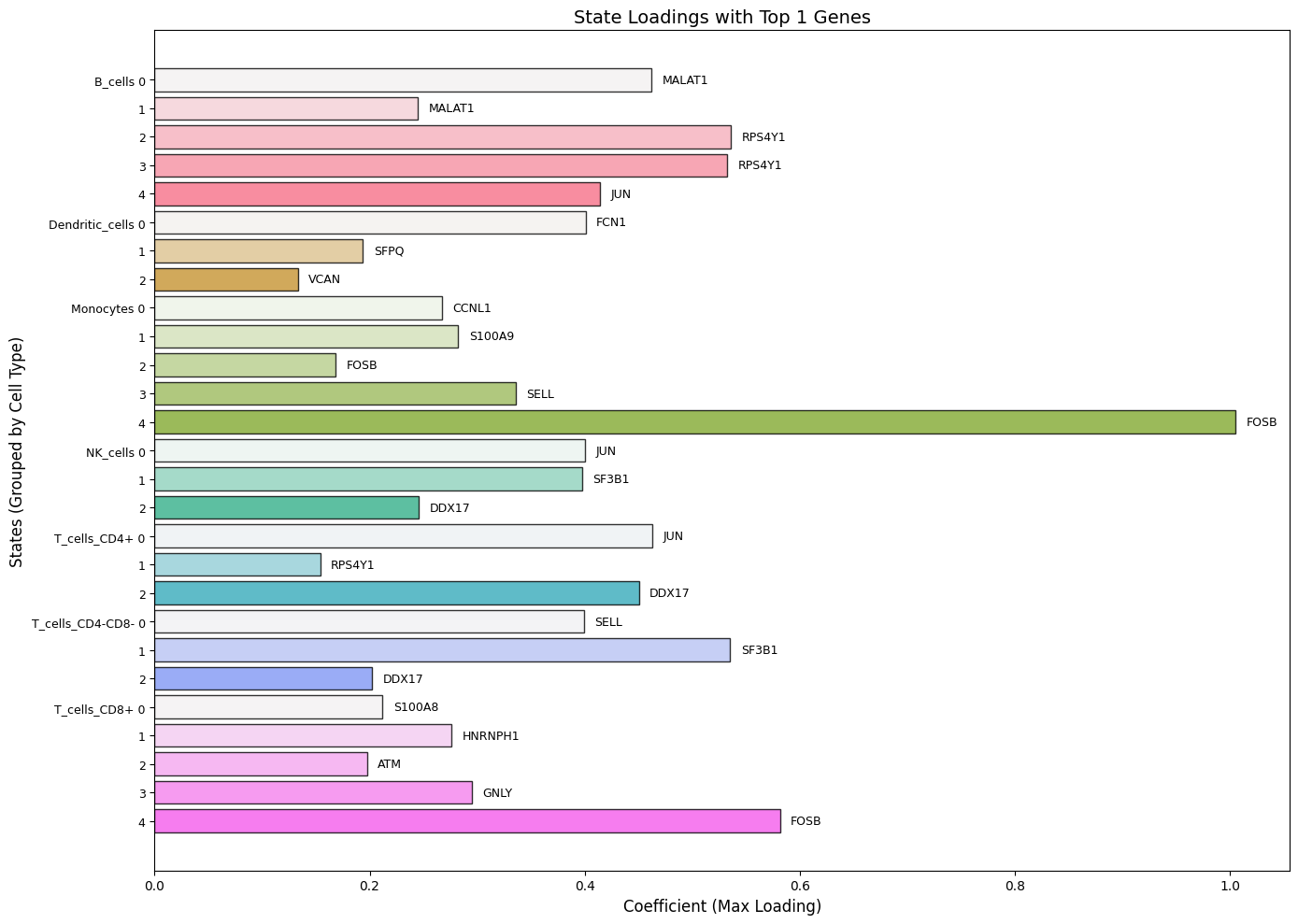
7.3: Bar Plot of State Loadings
from Statescope.Statescope import BarPlot_StateLoadings
BarPlot_StateLoadings(Statescope_model)
Console output: "StateLoadings matrix extracted successfully. Shape: (18638, 27)"